
On the first of July 2024 I successfully defended my PhD Thesis with the title Quasi Continuous Level Monte Carlo Method (1) and I am happy to share my work on the SFB-TRR 161 blog.
My PhD research focused on advancing stochastic simulation methods used in uncertainty quantification (UQ), specifically, improving the performance of Monte Carlo-based methods in their application to non-smooth stochastic problems. In my thesis I developed the Quasi Continuous Level Monte Carlo (QCLMC) method, a new algorithm that addresses fundamental challenges in preexisting methods. As computational simulations and UQ become increasingly important across industries, from engineering and finance to climate modeling and machine learning, the need for faster, more accurate, and scalable methods is ever-growing. Combining proven mathematical theory and practical performance the QCLMC method is a step towards meeting that need.
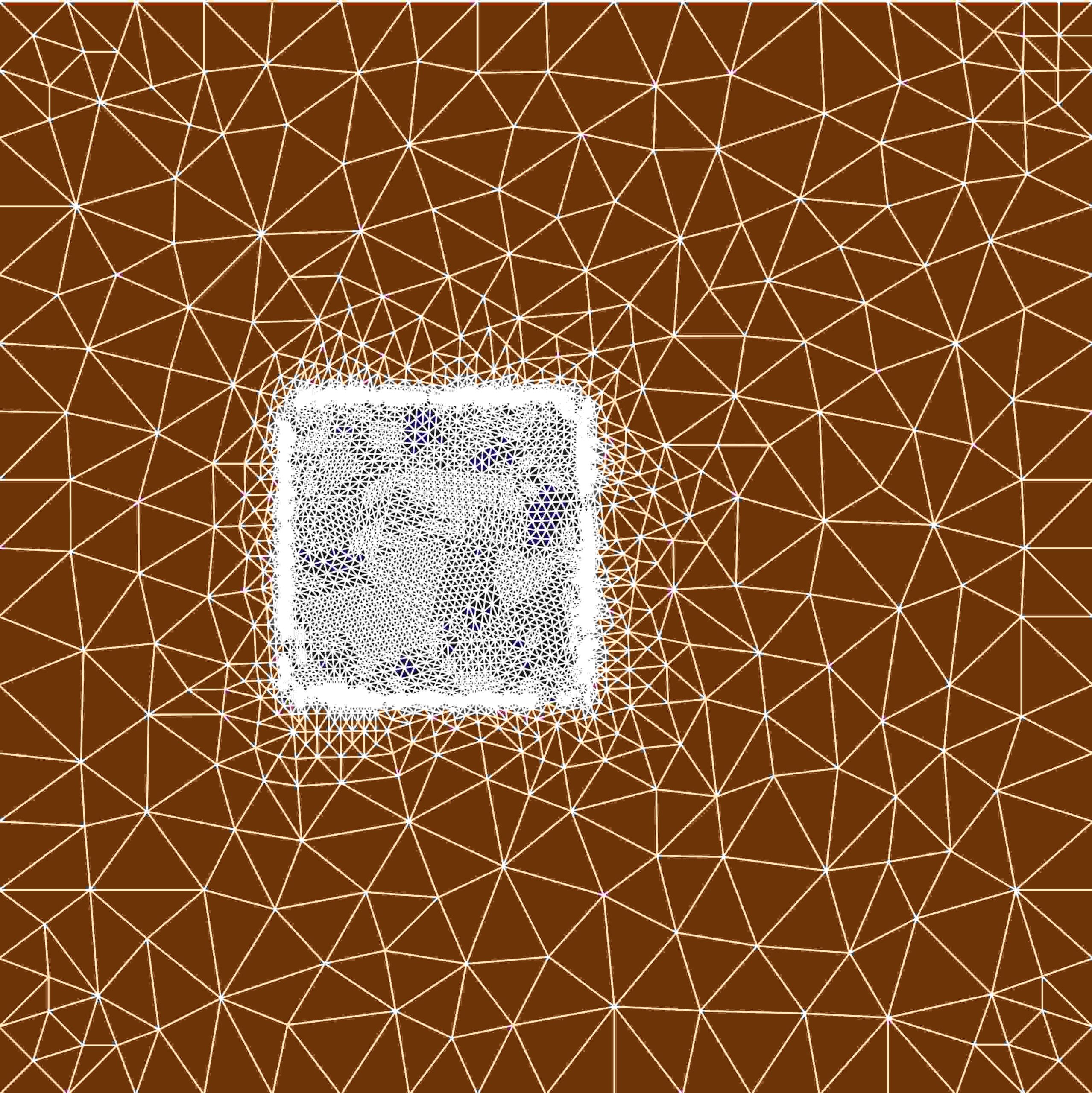
The construction of Stuttgart 21 yields a great example for the application of UQ in engineering and the environment. The drilling of train tunnels below Stuttgart is prone to uncertainty. Water may reach anhydrite stone layers of uncertain position and magnitude, see Figure 1. The anydrite stone can expand in volume significantly when coming in contact with water, potentially leading to the collision of tunnels or buildings above the surface. Mathematical models are used to circumvent these dangers by simulating the subsurface with its fractures and the involved uncertainties, see Figure 2. Adaptive computational methods are now required to simulate such models efficiently.
The Continuous Level Monte Carlo (CLMC) method (2) was recently developed as a flexible and general method for UQ. CLMC allows for the use of samplewise adaptive discretizations, e.g., adaptive finite elements (3), that naturally adapt to specific local features in samples of the stochastic problem at hand, e.g., anhydrite stone layers below Stuttgart, see Figure 1. Furthermore, CLMC is unbiased, meaning it can achieve the optimal time-to-error complexity without introducing systematic errors.


However, CLMC is not without its own challenges. While the method shows theoretical advantages, numerical experiments reveal that sampling the underlying level distribution, given by an exponential distribution, using independent identically distributed (i.i.d.) random samples can lead to a high variance in the estimator. This potentially increases the computational effort of the method in a way, which undermines its benefits.
My contribution: the Quasi Continuous Level Monte Carlo method
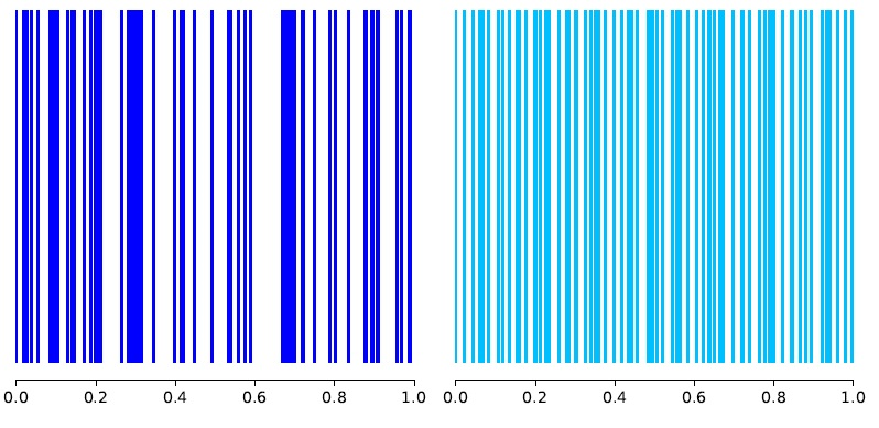
The main focus of my thesis was to resolve the high-variance issue in CLMC and to develop a more efficient method for practical applications. My work led to the development of the Quasi Continuous Level Monte Carlo (QCLMC) method, which leverages quasi-random numbers (5) instead of i.i.d. random samples to sample the underlying level distribution.
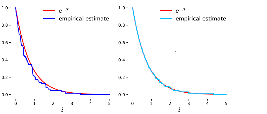
Quasi-random numbers are deterministic sequences with better distributional properties compared to i.i.d. random samples, see Figures 4 and 5. By using these sequences, QCLMC has a reduced variance while retaining the theoretical flexibility and adaptability of CLMC. Moreover, I proved that the QCLMC method is asymptotically unbiased and that it achieves the same asymptotic convergence rate as CLMC, but with a potentially lower computational cost.
Practical applications and numerical experiments
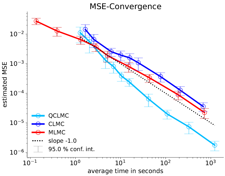
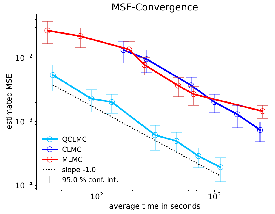
To ensure that these theoretical advancements translate into practical benefits, I developed routines to optimize the time-to-error performance for QCLMC and CLMC. This optimization allowed me to numerically compare the methods across a variety of scenarios including a simplified model for the Stuttgart 21 example given by a linear elliptic partial differential equation (PDE) with a discontinuous diffusion coefficient. The results were compelling. In every test case, QCLMC demonstrated practical optimality in terms of time-to-error performance, outperforming CLMC, see Figures 6 and 7.
Overall, my development of the QCLMC method contributes to the advancements in the field of stochastic simulations and UQ. By addressing the high-variance issue inherent in CLMC and introducing quasi-random sampling for the underlying level distribution, QCLMC offers a flexible, asymptotically unbiased and efficient approach to solving complex stochastic problems.
A big thank you goes to my colleagues in the UQ research group for creating a very pleasant working environment during my time at the university of Stuttgart, my advisor Andrea Barth for her great scientific support throughout and the DFG for funding my research within project B07 of the SFB-TRR 161.
If you’re working in fields that require heavy stochastic simulations or UQ, I encourage you to explore how QCLMC could benefit your work.
(1) C. A. Beschle, Quasi Continuous Level Monte Carlo Method, Dissertation, https://elib.uni-stuttgart.de/handle/11682/14942 , 2024.
(2) G. Detommaso, T. Dodwell, and R. Scheichl, Continuous level Monte Carlo and sampleadaptive model hierarchies, SIAM/ASA J. Uncertain. Quantif., 7, pp. 93-116.
https://doi.org/10.1137/18M1172259, 2019.
(3) T. Grätsch and K.-J. Bathe, A posteriori error estimation techniques in practical finite element analysis, Comput. & Structures, 83, pp. 235-265
https://doi.org/10.1016/j.compstruc.2004.08.011, 2005.
(4) D. Hägele, C. Schulz, C. A. Beschle, H. Booth, M. Butt, A. Barth, O. Deussen, D. Weiskopf: Uncertainty Visualization: Fundamentals and Recent Developments, in Info. Tech., https://doi.org/10.1515/itit-2022-0033, 2022.
(5) H. Niederreiter, Quasi-Monte Carlo methods and pseudo-random numbers, Bull. Amer. Math.Soc., 84 (1978), pp. 957-1041.
https://doi.org/10.1090/ 0002-9904-1978-14532-7.
(6) M. B. Giles, Multilevel Monte Carlo methods, Acta Numer., 24, pp. 259-328.
https://doi.org/10.1017/S096249291500001X, 2015.